Writing

SAM 3 찍먹 & 실전 활용 코드 정리

SAM 3를 직접 설치하고 추론 결과를 다루면서, 새 모델을 실제 파이프라인에 붙일 때 중요한 핸들링 포인트를 정리한 글.

Published Jan 6, 2026

1. 준비 작업 (Installation & Setup)

먼저 환경 설정입니다. Colab이나 로컬 환경에서 바로 돌려보실 수 있습니다. 최신 모델인 만큼 tfloat32와 bfloat16을 켜서 GPU 메모리를 아끼고 속도를 챙기는 것이 좋습니다.

import torch
import sys

# 1. 필수 라이브러리 설치
# (uv를 쓰신다면 uv add로 대체 가능합니다!)
# !{sys.executable} -m pip install opencv-python matplotlib scikit-learn
# !{sys.executable} -m pip install 'git+https://github.com/facebookresearch/sam3.git'

# 2. GPU 최적화 설정 (Ampere 아키텍처 이상 추천)
torch.backends.cuda.matmul.allow_tf32 = True
torch.backends.cudnn.allow_tf32 = True

# bfloat16 컨텍스트 설정 (메모리 절약)
torch.autocast("cuda", dtype=torch.bfloat16).__enter__()

필요 패키지 import

import os

import matplotlib.pyplot as plt
import numpy as np

import sam3
from PIL import Image
from sam3 import build_sam3_image_model
from sam3.model.box_ops import box_xywh_to_cxcywh
from sam3.model.sam3_image_processor import Sam3Processor
from sam3.visualization_utils import draw_box_on_image, normalize_bbox, plot_results

2. 모델 로드 및 이미지 준비

Hugging Face Hub 에 로그인하시어 SAM3모델의 토큰을 미리 준비해 주세요.

from huggingface_hub import login
login(token="여러분이 accpet 받으신 token")

그 다음,

# 모델 빌드 (경로는 본인 환경에 맞게 수정)
# bpe_path는 토크나이저 관련 파일입니다.
sam3_root = "..." # sam3 설치 경로
bpe_path = f"{sam3_root}/assets/bpe_simple_vocab_16e6.txt.gz"

model = build_sam3_image_model(bpe_path=bpe_path)

# 이미지 로드 및 전처리
image_path = "test_image.jpg" # 테스트할 이미지 경로
image = Image.open(image_path)

# 프로세서 초기화 (Confidence Threshold 조절 가능)
processor = Sam3Processor(model, confidence_threshold=0.5)
inference_state = processor.set_image(image)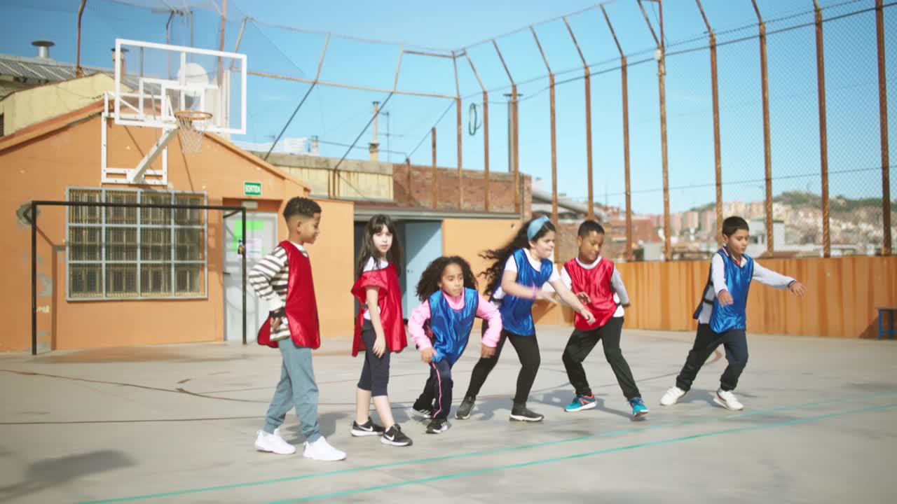

SAM3 원본 코드에서 제공하는 test_image.jpg이미지 입니다.

3. 프롬프트 추론 (Text & Box)

SAM 3의 장점은 자연어(str)나 박스 좌표(list)를 그냥 던져주면 알아서 찰떡같이 알아듣는다는 점입니다.

3.1 Text Prompt 예시

다양한 텍스트로 객체를 찾을 수 있습니다.

이번엔 예시로 "pants"를 찾아 보도록 하겠습니다.

# 텍스트로 객체 찾기
processor.reset_all_prompts(inference_state)
inference_state = processor.set_text_prompt(state=inference_state, prompt="pants")

img0 = Image.open(image_path)
plot_results(img0, inference_state)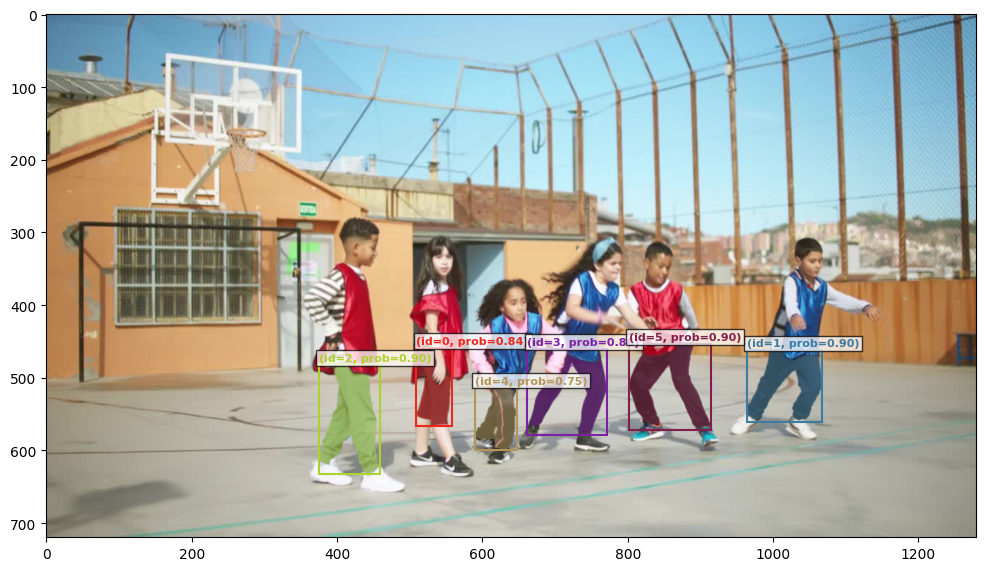

당연히 plot에서 bbox를 제거한 segmentation결과만 얻을 수도 있습니다.

3.2 BBOX 단수 입력 예시

이번엔 실제 bbox 좌표를 줘서 해당 부분과 같은 객체들을 segment 해보도록 하겠습니다.

입력이미지의 물리적 좌표의 bbox를 입력으로 넣고 추론을 합니다.

입력이미지의 물리적 좌표의 bbox가 prompt와 같은 역할을 한다고 이해하시면 됩니다.

# Here the box is in  (x,y,w,h) format, where (x,y) is the top left corner.
box_input_xywh = torch.tensor([480.0, 290.0, 110.0, 360.0]).view(-1, 4)
box_input_cxcywh = box_xywh_to_cxcywh(box_input_xywh)

norm_box_cxcywh = normalize_bbox(box_input_cxcywh, width, height).flatten().tolist()
print("Normalized box input:", norm_box_cxcywh)

processor.reset_all_prompts(inference_state)
inference_state = processor.add_geometric_prompt(
    state=inference_state, box=norm_box_cxcywh, label=True
)

img0 = Image.open(image_path)
image_with_box = draw_box_on_image(img0, box_input_xywh.flatten().tolist())
plt.imshow(image_with_box)
plt.axis("off")  # Hide the axis
plt.show()

box_input_xywh가 왼쪽에서 두번째 사람을 가르키는 것 입니다.

plot_results(img0, inference_state)

3.3 BBOX 복수 입력 예시

좀더 확장시켜 여러개의 bbox를 줄수도 있고 Positive & Negative option도 줄 수 있습니다.

box_input_xywh = [[480.0, 290.0, 110.0, 360.0], [370.0, 280.0, 115.0, 375.0]]
box_input_cxcywh = box_xywh_to_cxcywh(torch.tensor(box_input_xywh).view(-1,4))
norm_boxes_cxcywh = normalize_bbox(box_input_cxcywh, width, height).tolist()

box_labels = [True, False]

processor.reset_all_prompts(inference_state)

for box, label in zip(norm_boxes_cxcywh, box_labels):
    inference_state = processor.add_geometric_prompt(
        state=inference_state, box=box, label=label
    )

img0 = Image.open(image_path)
image_with_box = img0
for i in range(len(box_input_xywh)):
    if box_labels[i] == 1:
        color = (0, 255, 0)
    else:
        color = (255, 0, 0)
    image_with_box = draw_box_on_image(image_with_box, box_input_xywh[i], color)
plt.imshow(image_with_box)
plt.axis("off")  # Hide the axis
plt.show()

bbox단수입력과 마찬가지로 초록색 박스로 지정된 왼쪽에서 두번째와 같은 객체(=사람)을 찾아라 근데, 빨간색 박스로 지정된 왼쪽에서 첫번째는 제외해라

그 결과로!!

plot_results(img0, inference_state)

이를 활용하여 다양한 task를 진행해 볼 수 있지 않겠습니까? Meta가 베풀어주시는 copyleft의 은혜가 참으로 감사한 나날입니다.

4. [핵심] 결과 데이터 핸들링 (Practical Tips)

모델이 results라는 딕셔너리를 뱉어내는데, 여기서 우리가 실제로 필요한 Segmentation Mask를 끄집어내서 Numpy로 변환하는 과정이 제일 중요합니다. (실무에서 이 부분 때문에 에러가 많이 나죠.)

아래는 제가 사용하는 결과 처리 보일러플레이트 코드입니다.

Python

# 변수명이 results라고 가정합니다 (inference_state 혹은 predict 결과)

# (1) 마스크 키 찾기 (버전마다 키 값이 다를 수 있어 예외처리)
if 'pred_masks' in results:
    masks_tensor = results['pred_masks']
elif 'masks' in results:
    masks_tensor = results['masks']
else:
    print("마스크 키를 못 찾겠어요! keys:", results.keys())
    masks_tensor = None

if masks_tensor is not None:
    # (2) GPU 텐서 -> CPU Numpy 배열로 변환 (필수!)
    # .detach(): 그래디언트 계산 끊기
    # .cpu(): GPU 메모리에서 내리기
    # .numpy(): 넘파이 배열로 변환
    masks_np = masks_tensor.detach().cpu().numpy()

    # (3) Threshold 적용 (옵션)
    # SAM 결과는 보통 로짓(logit)값이므로 0보다 크면 마스크로 간주
    masks_np = masks_np > 0 
    
    print(f"Mask Shape: {masks_np.shape}")
    # 이후 OpenCV 등을 사용해 시각화하거나 저장하면 됩니다.

5. 마치며

직접 돌려보니 확실히 SAM 3가 이전 버전보다 멀티모달(텍스트+이미지) 이해도가 높아진 느낌입니다. 특히 pred_masks 텐서를 CPU로 내려서(detach().cpu().numpy()) 가공하는 부분만 주의하면, 기존 파이프라인에 바로 적용해 볼 수 있을 것 같습니다.

다음 포스팅에서는 이 SAM 3를 활용해 오토 라벨링(Auto-Labeling) 파이프라인을 구축하는 방법을 고민해 보겠습니다.

제가 진행하고 있는 프로젝트에 적용해 보았을때 정말 압도적인 성능을 보이고 있습니다.

Handy's Verdict:

"Segmentation의 끝판왕이 더 똑똑해져서 돌아왔습니다. 텍스트 프롬프트 기능은 진짜 물건이네요."